Armchair Transit with PostGIS: The Census & The Bestagons
June 28, 2026 • By Rhys • 12 min read
Kingston descended into gridlock on the afternoon of the 17th of April, 2026. Commuters of the Kingston Metropolitan Area (KMA) would not have foreseen the utter chaos they were destined to endure. Luckily, I was, on that day, a member of the set of human beings outside of the soon to be chaotic urban area.
If you followed social media, the cause of the congestion ranged from drivers not being courteous, to the insufficient road infrastructure. The fact that it was a Friday and there were heavy mid-afternoon showers1 may have also contributed to the mayhem. There were many reports of drivers spending in excess of three hours for what would nominally be a 45-minute commute. Personally, I think the obvious reason is that there are just too many cars on the island. Conversely, it is also obvious that the public transit system is woefully inadequate.
I am a fan of good public transport, and whenever I travel to other cities I often take a day or two to explore the transit. I sometimes even explore the city. I’m also a fan of the YouTube channels RMTransit and Not Just Bikes, channels that analyse and critique the transit systems of various cities. Transit punditry as it were. So, given that this blog is dedicated to all things spatial, you may have put 2 + 2 together and deduced that I’ll be trying to figure out how best to implement some kind of useful public transit for the KMA using some of my favourite spatial tools.
This will most likely be a multi-part series, the end goal: a proposed metro map for Kingston. Will it be a tram, a grade-separated system or a Bus Rapid Transit (BRT)? Likely none of those, as I think the Government of Jamaica (GoJ) lacks both the foresight and the money to make any kind of serious inroads to ameliorating this tragedy of transportation. Ok, let’s stick to technical stuff, I’ll reserve the right to make at most two more pseudo-political comments.
The first thing we need is data. We need to know where people live and how they get from place to place. Population and transportation. The GoJ’s most recent census was completed in 2022. Being staunch advocates of open data, they have seen fit to make this data publicly available for all to use. Let me clarify: they may have been staunch advocates as evidenced by the existence of data.gov.jm, but given the paucity of updates, I think they may have reconsidered. Did that count as a pseudo-political comment? Let’s cap it at 5. Nonetheless, the data I will be using is from the most recent census and is publicly available on a GoJ ArcGIS REST server. I just don’t know if they know it is published. For transportation, we will be using data from the good folks at the Overture Maps Foundation.
Setting up the database
Let us set up our database first. We are starting from scratch, a clean database named metro with no extensions installed. So let’s add our favourite spatial tool:
CREATE EXTENSION postgis;Next, we need a staging schema where we can load and check data before considering it gospel.
CREATE SCHEMA staging;This will be a mix of QGIS and PostGIS. I have the connection to the GoJ ArcGIS server in the QGIS browser. I’ll drag that into the canvas, visually inspect it to make sure it looks like Jamaica, then drag the layer into the staging schema using the browser tool. Lastly I will rename the table to census_2022. This census data is a list of Enumeration Districts (EDs) for the entirety of Jamaica.
Validating the data
The first rule of using data that you did not collect/map is to make sure it is sensible. You don’t want the analysis thrown off by dodgy data. The first check will be on the geometries. We like our data valid and simple.
SELECT st_isvalidreason(geom), st_issimple(geom), "ED", "ED_ID_1"
FROM staging.census_2022
WHERE NOT st_isvalid(geom) OR NOT st_issimple(geom);
┌────────────────────────────────────────────────────────────┬─────────────┬───────┬─────────┐
│ st_isvalidreason │ st_issimple │ ED │ ED_ID_1 │
╞════════════════════════════════════════════════════════════╪═════════════╪═══════╪═════════╡
│ Ring Self-intersection[-8553250.28588734 2044053.74059856] │ f │ WR 83 │ 212083 │
│ Ring Self-intersection[-8624347.55143995 2025932.05794956] │ f │ S 107 │ 1204107 │
└────────────────────────────────────────────────────────────┴─────────────┴───────┴─────────┘Two records have a “Ring Self-intersection”. PostGIS can attempt to fix them using the st_makevalid function. Let’s make sure that the function will return a valid geometry before we update the table.
WITH fixed AS (
    SELECT st_makevalid(geom) fixed, "ED" FROM staging.census_2022
    WHERE NOT st_isvalid(geom) OR NOT st_issimple(geom)
)
SELECT st_isvalid(fixed), st_issimple(fixed), "ED" FROM fixed;
┌────────────┬─────────────┬───────┐
│ st_isvalid │ st_issimple │ ED │
╞════════════╪═════════════╪═══════╡
│ t │ t │ WR 83 │
│ t │ t │ S 107 │
└────────────┴─────────────┴───────┘
Great! st_makevalid worked. And yes, if I can shoehorn a CTE into a query, I most certainly will. Let’s update the table.
UPDATE staging.census_2022
SET geom = st_makevalid(geom)
WHERE NOT st_isvalid(geom);
We could have done the update directly, but I would only recommend that if we were in a transaction block, that way if anything went awry, we could roll back to the previous state.
Our geometries are valid, let’s look at the actual data. Does the population total look right? Is the number of parishes correct?
SELECT
  sum("Population"), count(DISTINCT "PARISH"), string_agg(DISTINCT "PARISH", '|')
FROM staging.census_2022;
┌─────────┬───────┬───────────────────────────────────────────────────────────────────────────────────────────────────────────────────────────────────────────────────┐
│ sum │ count │ string_agg │
╞═════════╪═══════╪═══════════════════════════════════════════════════════════════════════════════════════════════════════════════════════════════════════════════════╡
│ 2774538 │ 14 │ CLARENDON|HANOVER|KINGSTON|MANCHESTER|PORTLAND|ST. ANDREW|ST. ANN|ST. CATHERINE|ST. ELIZABETH|ST. JAMES|ST. MARY|ST. THOMAS|TRELAWNY|WESTMORELAND │
└─────────┴───────┴───────────────────────────────────────────────────────────────────────────────────────────────────────────────────────────────────────────────────┘Yes. Both numbers look right and the parish names are recognizable. I have been waiting for Jamaica’s population to get to 3 million for some time now. I have long held the view that Jamaica is underpopulated, but this is a technical blog, not one for (more than 5) personal political views.
Looking at the column structure, it would appear that the PARISH, CONST and ED columns should form a naturally unique record identifier. Enumeration districts make up a constituency and constituencies constitute a parish.
SELECT
  "PARISH", "CONST", "ED", st_numgeometries(st_union(geom)), array_agg(st_numgeometries(geom)), count(*)
FROM staging.census_2022
GROUP BY 1, 2, 3
HAVING count(*) > 1;
┌───────────────┬──────────────┬────────┬──────────────────┬───────────┬───────┐
│ PARISH │ CONST │ ED │ st_numgeometries │ array_agg │ count │
╞═══════════════╪══════════════╪════════╪══════════════════╪═══════════╪═══════╡
│ CLARENDON │ SOUTH EAST │ SE 94 │ 1 │ {1,1} │ 2 │
│ ST. CATHERINE │ NORTH EAST │ NE 11 │ 1 │ {1,1} │ 2 │
│ ST. CATHERINE │ SOUTH WEST │ SW 126 │ 1 │ {1,1} │ 2 │
│ ST. CATHERINE │ WEST CENTRAL │ WC 86 │ 1 │ {1,1} │ 2 │
└───────────────┴──────────────┴────────┴──────────────────┴───────────┴───────┘Four rows (really eight records, since each row appears to be duplicated) fail that test. Given that in all cases, the st_union of the geometries returns a single geometry, the potential duplicates are at best contiguous (meaning neighbours that touch) or at worst actual geometric twins. In either case, compared to the total ED count, the number of errant records is quite small, so we can assume they won’t affect any downstream analysis. We will just work with the assumption that the population and dwelling figures for each ED are accurate. Let’s check if the ED_ID_1 column is unique; if not we will create another column.
SELECT count(*), count(DISTINCT "ED_ID_1") FROM staging.census_2022;┌───────┬───────┐
│ count │ count │
╞═══════╪═══════╡
│ 6611 │ 6611 │
└───────┴───────┘Success! So, we have what I would call a clean and valid dataset, with the exception of those potentially duplicated records that amount to less than 0.15% of the entire dataset.
Exit: Staging left
The next step is to create a schema to hold all the good data that we will work with and transfer this table to it. We will also rename some columns and convert the geometry column to Jamaica’s local CRS.
CREATE SCHEMA metro;
CREATE TABLE metro.census AS
SELECT
  "PARISH" parish,
  "CONST" constituency,
  "ED" enumeration_district,
  "ED_ID_1" ed,
  "COMM_ID" community_id,
  "COMM_NAME_" community,
  "DEV_AREA" development_area,
  "URBAN_AREA" urban_area,
  "ED_CLASS" ed_class,
  "URBAN_AR_1" urban_area_class,
  "Population" population,
  "Dwelling" dwellings,
  st_transform(geom, 3448)::geometry(Multipolygon, 3448) geom -- transform to JAD2001.
FROM staging.census_2022;

CREATE INDEX ON metro.census USING GIST (geom);
ALTER TABLE metro.census ADD PRIMARY KEY (ed);
The bestagons
We have our population data. What we want to do now is normalise it across the island. Enumeration districts come in all shapes and sizes. While that may be perfectly fine for collecting census data, it makes spatial analysis awkward because differences in population density can simply reflect differences in the size of the underlying polygons. By redistributing the data onto a uniform grid, every cell represents the same area, making hotspots much easier to compare visually and statistically. We’ll lose a little precision at the boundaries, but gain a much more consistent representation of population across the island. We will use hexagons (which are the bestagons) to standardise the population and dwelling counts. When it comes to standardised hexagons, you can’t get much better than Uber’s H3 project. But a DGGS2 is exactly the kind of overkill I don’t need. PostGIS has a lovely st_hexagongrid function that will suit our needs quite well. We just need to choose a size that, like the little bear’s porridge, is just right. I don’t want the grid too coarse as that would make finding areas where the population changes too difficult. Conversely, too fine and I’ll end up with hexagons representing individual people. I’m thinking 175 metres a side; 350 metres between opposing vertices. This figure sounds right. The good thing is, we can have all this in a single .sql file and rerun it with different values. No need to point and click your way through again if you need to make a change.
CREATE TABLE staging.hexagons AS
SELECT * FROM st_hexagongrid(
  175, box2d('MULTIPOINT(840000 615000, 600000 715000)'::geometry)
);

ALTER TABLE staging.hexagons
ALTER COLUMN geom TYPE geometry(Polygon, 3448)
USING st_setsrid(geom, 3448);

CREATE INDEX ON staging.hexagons USING GIST (geom);
The st_hexagongrid function’s second argument is the bounding box of the region you want the grid over. One would normally use the extent of the data they would be using the grid against, but yours truly is a bit odd. I like whole numbers, hence the very specific figures chosen above. The new table is void of any SRID info, so we use ALTER TABLE to add that info and finally we create an index on the hexagons.
Normalising population to the hex grid
Now that we have our grid we can normalise the population data onto it using a mixture of st_intersection, st_intersects and st_area. For clarity, when I say normalise the population data I mean to assign a population value to each hexagon. We take any arbitrary hexagon, determine which enumeration districts intersect it. Next, for each ED, we calculate the population density. Then we calculate the proportion of the hexagon that intersects that ED and use the area intersected to calculate the population in that part of the hexagon. Lastly we sum all those values and we get the population for that hexagon.
Here is an example using a single hexagon:
SELECT
i, j, ed,
st_area(st_intersection(h.geom, p.geom)) area_intersected,
st_area(p.geom) area_of_ed,
population / st_area(p.geom) pop_density,
st_area(st_intersection(h.geom, p.geom)) * (population / st_area(p.geom)) population_intersected,
population
FROM staging.hexagons h
JOIN metro.census p ON st_intersects(p.geom, h.geom)
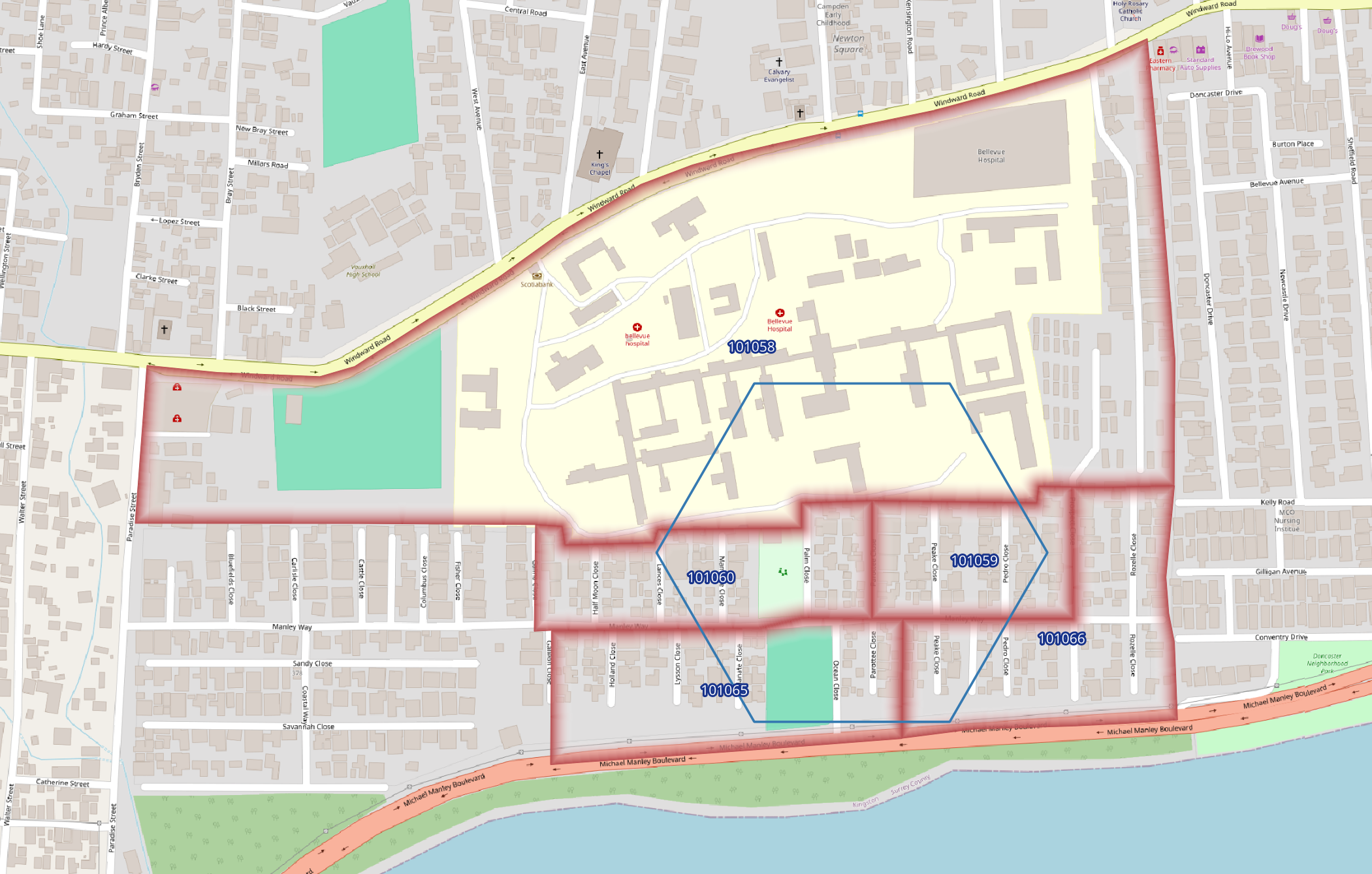
WHERE i = 2950 AND j = 2133;It intersects 5 EDs and you can see the last column has a figure that represents the population allocated to the intersected portion of each ED.
┌──────┬──────┬────────┬────────────────────┬────────────────────┬────────────┬────────────────────────┐
│  i   │  j   │   ed   │  area_intersected  │    area_of_ed      │ population │ population_intersected │
╞══════╪══════╪════════╪════════════════════╪════════════════════╪════════════╪════════════════════════╡
│ 2950 │ 2133 │ 101058 │ 27811.845774119596 │ 250085.85845470292 │       1571 │      174.7096376465274 │
│ 2950 │ 2133 │ 101066 │  6308.397963303272 │ 33998.291805069355 │        322 │      59.74724129759877 │
│ 2950 │ 2133 │ 101059 │ 14831.491350785596 │ 19266.395746515263 │        312 │      240.1811611433381 │
│ 2950 │ 2133 │ 101060 │ 16552.664450761513 │  26843.86533963807 │        468 │     288.58165040477866 │
│ 2950 │ 2133 │ 101065 │ 14061.684433736726 │ 35524.089258277214 │        373 │     147.64652390241636 │
└──────┴──────┴────────┴────────────────────┴────────────────────┴────────────┴────────────────────────┘
And here is what that looks like:
The final query sums the population and dwelling values for each hexagon across all intersecting EDs:
CREATE TABLE metro.hex_census AS
SELECT
  i, j,
  sum(st_area(st_intersection(h.geom, p.geom)) * (population / st_area(p.geom))) population,
  sum(st_area(st_intersection(h.geom, p.geom)) * (dwellings / st_area(p.geom))) dwellings,
  h.geom
FROM staging.hexagons h
JOIN metro.census p ON st_intersects(p.geom, h.geom)
GROUP BY i, j, h.geom;

ALTER TABLE metro.hex_census ADD PRIMARY KEY (i, j);
CREATE INDEX ON metro.hex_census USING GIST (geom);
And here is what that data looks like:
Let’s take off the data wrangling hat and put on the urban planning hat; to be honest, I’m moving from a sombrero or fedora to a beret or beanie. My knowledge in this arena is sparse. Nonetheless, we can make some astute observations about Kingston based on the data. What jumps out to me is the corridor of higher density (the deepest reds) running from downtown Kingston northwest, roughly aligned with Spanish Town Road. A metro wants to thread the densest areas and this, I think, would definitely be a corridor where stations would be needed. Portmore (just west of Kingston across Hunt’s Bay) also cannot be left out. Any proposed metro would have to connect the two. But, this data only shows where people live, not where they work. The whole point of transit is to get folks to where they want to be. This is where the Overture data may come in handy. Who knows, maybe that public GoJ server has data that may be useful as well.
Recap
To recap: we grabbed some population data from the GoJ’s ArcGIS server, validated and cleaned the geometries, created a hexagon grid across the island, then used some straightforward spatial functions to normalise the population and dwelling data onto the hex grid.
The next post will look at where the demand for transport is. Step one in the quest for good transit in Kingston is complete.
A quick count(*) on my pseudo-political comments puts us at four, one under budget. I’ll carry the remainder forward to Part 2.